Pileups and average features

Welcome to the cooltools pileups notebook!

Averaging Hi-C/Micro-C maps allows the quantification of general patterns observed in the maps. Averaging comes in various forms: contact-vs-distance plots, saddle plots, and pileup plots. Pileup plots are the averaged local Hi-C map over the 2D windows (i.e. snippets). These are also referred to as “average Hi-C maps”. Pileups can be useful for determining the relationship between features (e.g. CTCF and TAD boundaries). Pileups can also be beneficial for reliably observing features in low-coverage Hi-C or single-cell HiC maps.

For pileups, we retrieve local windows that are centered at the anchors. We call this procedure snipping. Anchors can be ChIP-Seq binding sites, anchors of dots, or any other genomic features. Pileups come in two varieties:

• On-diagonal pileup. Each window is centered at the pixel located at the anchor position, at the main diagonal. Both coordinates of the window center are equivalent to the bin of the anchor.

• Off-diagonal pileup. Each window is centered at the pixel with one anchor as a left coordinate and another anchor as a right coordinate.

Typically, the sizes of windows are equivalent. After the selection of windows, we average them elementwise.

Content:

1. Download data

2. Load data

   • Load genomic regions

   • Load features for anchors

3. On-diagonal pipeup of CTCF

   • On-diagonal pileup of ICed Hi-C interactions

   • On-diagonal pileup of observed over expected interactions

   • Inspect the snips

4. Off-diagonal pileup of CTCF

# If you are a developer, you may want to reload the packages on a fly.
# Jupyter has a magic for this particular purpose:
%load_ext autoreload
%autoreload 2

# import standard python libraries
import numpy as np
import matplotlib.pyplot as plt
import pandas as pd
import seaborn as sns

# import libraries for biological data analysis
import cooler
import bioframe

import cooltools

from packaging import version
if version.parse(cooltools.__version__) < version.parse('0.5.2'):
    raise AssertionError("tutorials rely on cooltools version 0.5.2 or higher,"+
                         "please check your cooltools version and update to the latest")

Download data

For this example notebook, we collected the data from immortalized human foreskin fibroblast cell line HFFc6:

• Micro-C data from Krietenstein et al. 2020

• ChIP-Seq for CTCF from ENCODE ENCSR000DWQ

You can automatically download test datasets with cooltools. More information on the files and how they were obtained is available from the datasets description.

# Print available datasets for download
cooltools.print_available_datasets()

1) HFF_MicroC : Micro-C data from HFF human cells for two chromosomes (hg38) in a multi-resolution mcool format.
        Downloaded from https://osf.io/3h9js/download
        Stored as test.mcool
        Original md5sum: e4a0fc25c8dc3d38e9065fd74c565dd1

2) HFF_CTCF_fc : ChIP-Seq fold change over input with CTCF antibodies in HFF cells (hg38). Downloaded from ENCODE ENCSR000DWQ, ENCFF761RHS.bigWig file
        Downloaded from https://osf.io/w92u3/download
        Stored as test_CTCF.bigWig
        Original md5sum: 62429de974b5b4a379578cc85adc65a3

3) HFF_CTCF_binding : Binding sites called from CTCF ChIP-Seq peaks for HFF cells (hg38). Peaks are from ENCODE ENCSR000DWQ, ENCFF498QCT.bed file. The motifs are called with gimmemotifs (options --nreport 1 --cutoff 0), with JASPAR pwm MA0139.
        Downloaded from https://osf.io/c9pwe/download
        Stored as test_CTCF.bed.gz
        Original md5sum: 61ecfdfa821571a8e0ea362e8fd48f63

# Downloading test data for pileups
# cache = True will doanload the data only if it was not previously downloaded
data_dir = './data/'
cool_file = cooltools.download_data("HFF_MicroC", cache=True, data_dir=data_dir)
ctcf_peaks_file = cooltools.download_data("HFF_CTCF_binding", cache=True, data_dir=data_dir)
ctcf_fc_file = cooltools.download_data("HFF_CTCF_fc", cache=True, data_dir=data_dir)

Load data

Load genomic regions

The pileup function needs genomic regions. Why?

• First, pileup uses regions for parallelization of snipping. Different genomic regions are loaded simultaneously by different processes, and the snipping can be done in parallel.

• Second, the observed over expected pileup requires calculating expected interactions before snipping (P(s), in other words). Typically, P(s) is calculated separately for each chromosome arm as inter-arms interactions might be affected by strong insulation of centromeres or Rabl configuration.

For species that do not have information on chromosome arms, or have telocentric chromosomes (e.g., mouse), you may want to use full chromosomes instead.

# Open cool file with Micro-C data:
clr = cooler.Cooler(data_dir+'/test.mcool::/resolutions/10000')
# Set up selected data resolution:
resolution = clr.binsize

# Use bioframe to fetch the genomic features from the UCSC.
hg38_chromsizes = bioframe.fetch_chromsizes('hg38')
hg38_cens = bioframe.fetch_centromeres('hg38')
hg38_arms = bioframe.make_chromarms(hg38_chromsizes, hg38_cens)

# Select only chromosomes that are present in the cooler.
# This step is typically not required! we call it only because the test data are reduced.
hg38_arms = hg38_arms.set_index("chrom").loc[clr.chromnames].reset_index()

Load features for anchors

Construction of the pileup requires genomic features that will be used for centering of the snippets. In this example, we will use positions of motifs in CTCF peaks as features.

# Read CTCF peaks data and select only chromosomes present in cooler:
ctcf = bioframe.read_table(ctcf_peaks_file, schema='bed').query(f'chrom in {clr.chromnames}')
ctcf['mid'] = (ctcf.end+ctcf.start)//2
ctcf.head()

	chrom	start	end	name	score	strand	mid
17271	chr17	118485	118504	MA0139.1_CTCF_human	12.384042	-	118494
17272	chr17	144002	144021	MA0139.1_CTCF_human	11.542617	+	144011
17273	chr17	163676	163695	MA0139.1_CTCF_human	5.294219	-	163685
17274	chr17	164711	164730	MA0139.1_CTCF_human	11.889376	+	164720
17275	chr17	309416	309435	MA0139.1_CTCF_human	7.879575	-	309425

Feature inspection and filtering

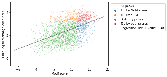
Since we have both the list of strongest motifs of CTCF located in CTCF ChIP-Seq and the fold change over input for the genome, we have two characteristics of each feature:

• score of the motif

• CTCF ChIP-Seq fold-change over input

Let’s take a look at joint distribution of these scores:

import bbi
from scipy.stats import linregress

# Get CTCF ChIP-Seq fold-change over input for genomic regions centered at the positions of the motifs

flank = 250 # Length of flank to one side from the boundary, in basepairs
ctcf_chip_signal = bbi.stackup(
    ctcf_fc_file,
    ctcf.chrom,
    ctcf.mid-flank,
    ctcf.mid+flank,
    bins=1)

ctcf['FC_score'] = ctcf_chip_signal

ctcf['quartile_score']    = pd.qcut(ctcf['score'], 4, labels=False) + 1
ctcf['quartile_FC_score'] = pd.qcut(ctcf['FC_score'], 4, labels=False) + 1
ctcf['peaks_importance'] = ctcf.apply(
    lambda x: 'Top by both scores' if x.quartile_score==4 and x.quartile_FC_score==4 else
                'Top by Motif score' if x.quartile_score==4 else
                'Top by FC score' if x.quartile_FC_score==4 else 'Ordinary peaks', axis=1
)

x = ctcf['score']
y = np.log(ctcf['FC_score'])

fig, ax = plt.subplots()

sns.scatterplot(x=x, y=y, hue=ctcf['peaks_importance'],
    s=2,
    alpha=0.5,
    label='All peaks',
    ax=ax
)

slope, intercept, r, p, se = linregress(x, y)

ax.plot([-6, 19], [intercept-6*slope, intercept+19*slope],
        alpha=0.5,
        color='black',
        label=f"Regression line, R value: {r:.2f}")

ax.set(
    xlabel='Motif score',
    ylabel='ChIP-Seq fold-change over input')

ax.legend(bbox_to_anchor=(1.01,1), loc="upper left")

plt.show()

/Users/geofffudenberg/anaconda3/envs/open2c/lib/python3.8/site-packages/seaborn/_decorators.py:36: FutureWarning: Pass the following variables as keyword args: x, y. From version 0.12, the only valid positional argument will be `data`, and passing other arguments without an explicit keyword will result in an error or misinterpretation.
  warnings.warn(

# Select the CTCF sites that are in top quartile by both the ChIP-Seq data and motif score

sites = ctcf[ctcf['peaks_importance']=='Top by both scores']\
    .sort_values('FC_score', ascending=False)\
    .reset_index(drop=True)
sites.tail()

	chrom	start	end	name	score	strand	mid	FC_score	quartile_score	quartile_FC_score	peaks_importance
659	chr17	8158938	8158957	MA0139.1_CTCF_human	13.276979	-	8158947	25.056849	4	4	Top by both scores
660	chr2	176127201	176127220	MA0139.1_CTCF_human	12.820343	+	176127210	25.027294	4	4	Top by both scores
661	chr17	38322364	38322383	MA0139.1_CTCF_human	13.534864	-	38322373	25.010430	4	4	Top by both scores
662	chr2	119265336	119265355	MA0139.1_CTCF_human	13.739862	-	119265345	24.980141	4	4	Top by both scores
663	chr2	118003514	118003533	MA0139.1_CTCF_human	12.646685	-	118003523	24.957502	4	4	Top by both scores

# Some CTCF sites might be located too close in the genome and interfere with analysis.
# We will collapse the sites falling into the same size genomic bins as the resolution of our micro-C data:
sites = bioframe.cluster(sites, min_dist=resolution)\
    .drop_duplicates('cluster')\
    .reset_index(drop=True)
sites.tail()

	chrom	start	end	name	score	strand	mid	FC_score	quartile_score	quartile_FC_score	peaks_importance	cluster	cluster_start	cluster_end
608	chr17	8158938	8158957	MA0139.1_CTCF_human	13.276979	-	8158947	25.056849	4	4	Top by both scores	34	8158938	8158957
609	chr2	176127201	176127220	MA0139.1_CTCF_human	12.820343	+	176127210	25.027294	4	4	Top by both scores	515	176127201	176127220
610	chr17	38322364	38322383	MA0139.1_CTCF_human	13.534864	-	38322373	25.010430	4	4	Top by both scores	104	38322364	38322383
611	chr2	119265336	119265355	MA0139.1_CTCF_human	13.739862	-	119265345	24.980141	4	4	Top by both scores	465	119265336	119265355
612	chr2	118003514	118003533	MA0139.1_CTCF_human	12.646685	-	118003523	24.957502	4	4	Top by both scores	462	118003514	118003533

On-diagonal pileup

On-diagonal pileup is the simplest, you need the positions of features (middlepoints of CTCF motifs) and the size of flanks aroung each motif. cooltools will create a snippet of Hi-C map for each feature. Then you can combine them into a single 2D pileup.

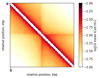
On-diagonal pileup of ICed Hi-C interactions

stack = cooltools.pileup(clr, sites, view_df=hg38_arms, flank=300_000)
# Mirror reflect snippets when the feature is on the opposite strand
mask = np.array(sites.strand == '-', dtype=bool)
stack[:, :, mask] = stack[::-1, ::-1, mask]

# Aggregate. Note that some pixels might be converted to NaNs after IC, thus we aggregate by nanmean:
mtx = np.nanmean(stack, axis=2)

# Load colormap with large number of distinguishable intermediary tones,
# The "fall" colormap in cooltools is exactly for this purpose.
# After this step, you can use "fall" as cmap parameter in matplotlib:
import cooltools.lib.plotting

plt.imshow(
    np.log10(mtx),
    vmin = -3,
    vmax = -1,
    cmap='fall',
    interpolation='none')

plt.colorbar(label = 'log10 mean ICed Hi-C')
ticks_pixels = np.linspace(0, flank*2//resolution,5)
ticks_kbp = ((ticks_pixels-ticks_pixels[-1]/2)*resolution//1000).astype(int)
plt.xticks(ticks_pixels, ticks_kbp)
plt.yticks(ticks_pixels, ticks_kbp)
plt.xlabel('relative position, kbp')
plt.ylabel('relative position, kbp')

plt.show()

/var/folders/4s/d866wm3s4zbc9m41334fxfwr0000gp/T/ipykernel_33615/2426526626.py:2: RuntimeWarning: divide by zero encountered in log10
  np.log10(mtx),

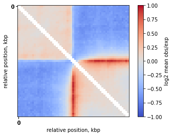
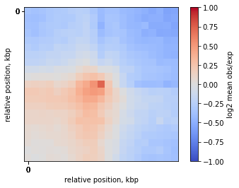
On-diagonal pileup of observed over expected interactions

Sometimes you don’t want to include the distance decay P(s) in your pileups. For example, when you make comparison of pileups between experiments and they have different P(s). Even if these differences are slight, they might affect the pileup of raw ICed Hi-C interactions.

In this case, the observed over expected pileup is your choice. Prior to running the pileup function, you need to calculate expected interactions for chromosome arms.

expected = cooltools.expected_cis(clr, view_df=hg38_arms, nproc=2, chunksize=1_000_000)

expected

	region1	region2	dist	n_valid	count.sum	balanced.sum	count.avg	balanced.avg	balanced.avg.smoothed	balanced.avg.smoothed.agg
0	chr2_p	chr2_p	0	8771	NaN	NaN	NaN	NaN	NaN	NaN
1	chr2_p	chr2_p	1	8753	NaN	NaN	NaN	NaN	0.000495	0.000520
2	chr2_p	chr2_p	2	8745	2656738.0	406.013088	303.800800	0.046428	0.042469	0.044728
3	chr2_p	chr2_p	3	8741	1563363.0	237.585271	178.854021	0.027181	0.026796	0.028226
4	chr2_p	chr2_p	4	8738	1125674.0	169.308714	128.825132	0.019376	0.019097	0.020152
...	...	...	...	...	...	...	...	...	...	...
32543	chr17_q	chr17_q	5850	0	0.0	0.000000	NaN	NaN	0.000010	0.000006
32544	chr17_q	chr17_q	5851	0	0.0	0.000000	NaN	NaN	0.000010	0.000006
32545	chr17_q	chr17_q	5852	0	0.0	0.000000	NaN	NaN	0.000010	0.000006
32546	chr17_q	chr17_q	5853	0	0.0	0.000000	NaN	NaN	0.000010	0.000006
32547	chr17_q	chr17_q	5854	0	0.0	0.000000	NaN	NaN	0.000010	0.000006

32548 rows × 10 columns

# Create the stack of snips:
stack = cooltools.pileup(clr, sites, view_df=hg38_arms, expected_df=expected, flank=300_000)

# Mirror reflect snippets when the feature is on the opposite strand
mask = np.array(sites.strand == '-', dtype=bool)
stack[:, :, mask] = stack[::-1, ::-1, mask]

mtx = np.nanmean(stack, axis=2)

plt.imshow(
    np.log2(mtx),
    vmax = 1.0,
    vmin = -1.0,
    cmap='coolwarm',
    interpolation='none')

plt.colorbar(label = 'log2 mean obs/exp')
ticks_pixels = np.linspace(0, flank*2//resolution,5)
ticks_kbp = ((ticks_pixels-ticks_pixels[-1]/2)*resolution//1000).astype(int)
plt.xticks(ticks_pixels, ticks_kbp)
plt.yticks(ticks_pixels, ticks_kbp)
plt.xlabel('relative position, kbp')
plt.ylabel('relative position, kbp')

plt.show()

/var/folders/4s/d866wm3s4zbc9m41334fxfwr0000gp/T/ipykernel_33615/2557000624.py:2: RuntimeWarning: divide by zero encountered in log2
  np.log2(mtx),

Inspect the snips

Aggregation is a convenient though dangerous step. It averages your data so that you cannot distinguish whether the signal is indeed average, or there is a single dataset that introduces a bias to your analysis. To make sure there are no outliers, you may want to use inspection of individual snippets.

The cell below shows one way to interactively investigate snippets contributing to a pileup. Note that this is not interactive on readthedocs, but can be run if the notebook is obtained from open2c_examples. This widget sorts the dataframe with CTCF motifs by the strength of binding. This allows us to inspect the Micro-C maps at the positions of the strongest and weakest CTCF sites. Run the cell below and try to compare snippets with the lowest score to the snippets with the largest score.

from ipywidgets import interact
from matplotlib.gridspec import GridSpec

n_examples = len(sites)

@interact(i=(0, n_examples-1))
def f(i):
    fig, ax = plt.subplots(figsize=[5,5])
    img = ax.matshow(
        np.log2(stack[:, :, i]),
        vmin=-1,
        vmax=1,
        extent=[-flank//1000, flank//1000, -flank//1000, flank//1000],
        cmap='coolwarm'
    )
    ax.xaxis.tick_bottom()
    if i > 0:
        ax.yaxis.set_visible(False)
    plt.title(f'{i+1}-th snippet from top \n FC score: {sites.loc[i, "FC_score"]:.2f}\n and motif score: {sites.loc[i, "score"]:.2f}')
    plt.axvline(0, c='g', ls=':')
    plt.axhline(0, c='g', ls=':')

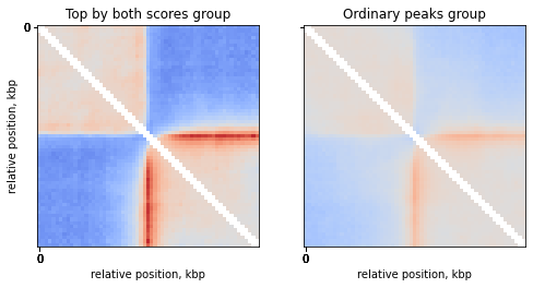
Compare top strongest peaks with others

Compare the top peaks with both motif score and FC score to the rest of the peaks:

# Create the stack of snips:
stack = cooltools.pileup(clr, ctcf, view_df=hg38_arms, expected_df=expected, flank=300_000
            )

# Mirror reflect snippets where the feature is on the opposite strand
mask = np.array(ctcf.strand == '-', dtype=bool)
stack[:, :, mask] = stack[::-1, ::-1, mask]

mtx = np.nanmean(stack, axis=2)

# TODO: add some strength of insulation for the pileup?

groups = ['Top by both scores', 'Ordinary peaks']
n_groups = len(groups)

ticks_pixels = np.linspace(0, flank*2//resolution,5)
ticks_kbp = ((ticks_pixels-ticks_pixels[-1]/2)*resolution//1000).astype(int)

fig, axs = plt.subplots(1, n_groups, sharex=True, sharey=True, figsize=(4*n_groups, 4))
for i in range(n_groups):
    mtx = np.nanmean( stack[:, :, ctcf['peaks_importance']==groups[i]], axis=2)
    ax = axs[i]
    ax.imshow(
        np.log2(mtx),
        vmax = 1.0,
        vmin = -1.0,
        cmap='coolwarm',
        interpolation='none')

    ax.set(title=f'{groups[i]} group',
           xticks=ticks_pixels,
           xticklabels=ticks_kbp,
           xlabel='relative position, kbp')

axs[0].set(yticks=ticks_pixels,
       yticklabels=ticks_kbp,
       ylabel='relative position, kbp')

plt.show()

/var/folders/4s/d866wm3s4zbc9m41334fxfwr0000gp/T/ipykernel_33615/2210978640.py:14: RuntimeWarning: divide by zero encountered in log2
  np.log2(mtx),

Off-diagonal pileup

Off-diagonal pileups are the averaged Hi-C maps around double anchors. In this case, the anchors are CTCF sites in the genome.

paired_sites = bioframe.pair_by_distance(sites, min_sep=200000, max_sep=1000000, suffixes=('1', '2'))
paired_sites.loc[:, 'mid1'] = (paired_sites['start1'] + paired_sites['end1'])//2
paired_sites.loc[:, 'mid2'] = (paired_sites['start2'] + paired_sites['end2'])//2

print(len(paired_sites))
paired_sites.head()

1634

	chrom1	start1	end1	name1	score1	strand1	mid1	FC_score1	quartile_score1	quartile_FC_score1	...	score2	strand2	mid2	FC_score2	quartile_score2	quartile_FC_score2	peaks_importance2	cluster2	cluster_start2	cluster_end2
0	chr17	412407	412426	MA0139.1_CTCF_human	12.212548	+	412416	41.645123	4	4	...	13.272118	-	1056231	35.072572	4	4	Top by both scores	1	1056222	1056241
1	chr17	412407	412426	MA0139.1_CTCF_human	12.212548	+	412416	41.645123	4	4	...	13.996208	-	1187374	69.994562	4	4	Top by both scores	2	1187365	1187384
2	chr17	412407	412426	MA0139.1_CTCF_human	12.212548	+	412416	41.645123	4	4	...	14.735101	+	1259280	31.643758	4	4	Top by both scores	3	1259271	1259290
3	chr17	412407	412426	MA0139.1_CTCF_human	12.212548	+	412416	41.645123	4	4	...	13.983562	+	1276338	35.440247	4	4	Top by both scores	4	1276329	1276348
4	chr17	412407	412426	MA0139.1_CTCF_human	12.212548	+	412416	41.645123	4	4	...	12.045221	+	1365609	36.746886	4	4	Top by both scores	5	1365600	1365619

5 rows × 28 columns

For pileup, we will use the expected calculated above:

# create the stack of snips:
stack = cooltools.pileup(clr, paired_sites, view_df=hg38_arms, expected_df=expected, flank=100_000)

mtx = np.nanmean(stack, axis=2)

plt.imshow(
    np.log2(mtx),
    vmax = 1,
    vmin = -1,
    cmap='coolwarm')

plt.colorbar(label = 'log2 mean obs/exp')
ticks_pixels = np.linspace(0, flank*2//resolution,5)
ticks_kbp = ((ticks_pixels-ticks_pixels[-1]/2)*resolution//1000).astype(int)
plt.xticks(ticks_pixels, ticks_kbp)
plt.yticks(ticks_pixels, ticks_kbp)
plt.xlabel('relative position, kbp')
plt.ylabel('relative position, kbp')

plt.show()

---

This page was generated with nbsphinx from /home/docs/checkouts/readthedocs.org/user_builds/cooltools/checkouts/latest/docs/notebooks/pileup_CTCF.ipynb