Command line interface
Welcome to the cooltools command line interface (CLI) notebook!
Cooltools features a paired python API & CLI that enables user-facing functions to be run from the command line.
[1]:
import os, subprocess
import pandas as pd
import bioframe
import cooltools
import cooler
import numpy as np
import matplotlib.pyplot as plt
from matplotlib.colors import LogNorm
plt.rcParams['font.size']=12

from packaging import version
if version.parse(cooltools.__version__) < version.parse('0.5.2'):
    raise AssertionError("tutorials rely on cooltools version 0.5.2 or higher,"+
                         "please check your cooltools version and update to the latest")

# We can use this function to display a file within the notebook
from IPython.display import Image


# download test data
# this file is 145 Mb, and may take a few seconds to download
cool_file = cooltools.download_data("HFF_MicroC", cache=True, data_dir='./data/')
print(cool_file)

# To use this variable in a bash call from jupyter just use $cool_file
./data/test.mcool
[2]:
%%bash
mkdir -p data
mkdir -p outputs
[3]:
# Note for the correct bash environment to be recognized from jupyter with the ! magic,
# jupyter notebook must be initialized from a conda environment with cooler and cooltools installed.
To see a list of CLI commands for cooltools, see the help:
[4]:
!cooltools -h
Usage: cooltools [OPTIONS] COMMAND [ARGS]...

  Type -h or --help after any subcommand for more information.

Options:
  -v, --verbose  Verbose logging
  -d, --debug    Post mortem debugging
  -V, --version  Show the version and exit.
  -h, --help     Show this message and exit.

Commands:
  coverage        Calculate the sums of cis and genome-wide contacts (aka...
  dots            Call dots on a Hi-C heatmap that are not larger than...
  eigs-cis        Perform eigen value decomposition on a cooler matrix to...
  eigs-trans      Perform eigen value decomposition on a cooler matrix to...
  expected-cis    Calculate expected Hi-C signal for cis regions of...
  expected-trans  Calculate expected Hi-C signal for trans regions of...
  genome          Utilities for binned genome assemblies.
  insulation      Calculate the diamond insulation scores and call...
  pileup          Perform retrieval of the snippets from .cool file.
  random-sample   Pick a random sample of contacts from a Hi-C map.
  saddle          Calculate saddle statistics and generate saddle plots...
  virtual4c       Generate virtual 4C profile from a contact map by...
Visualization
[5]:
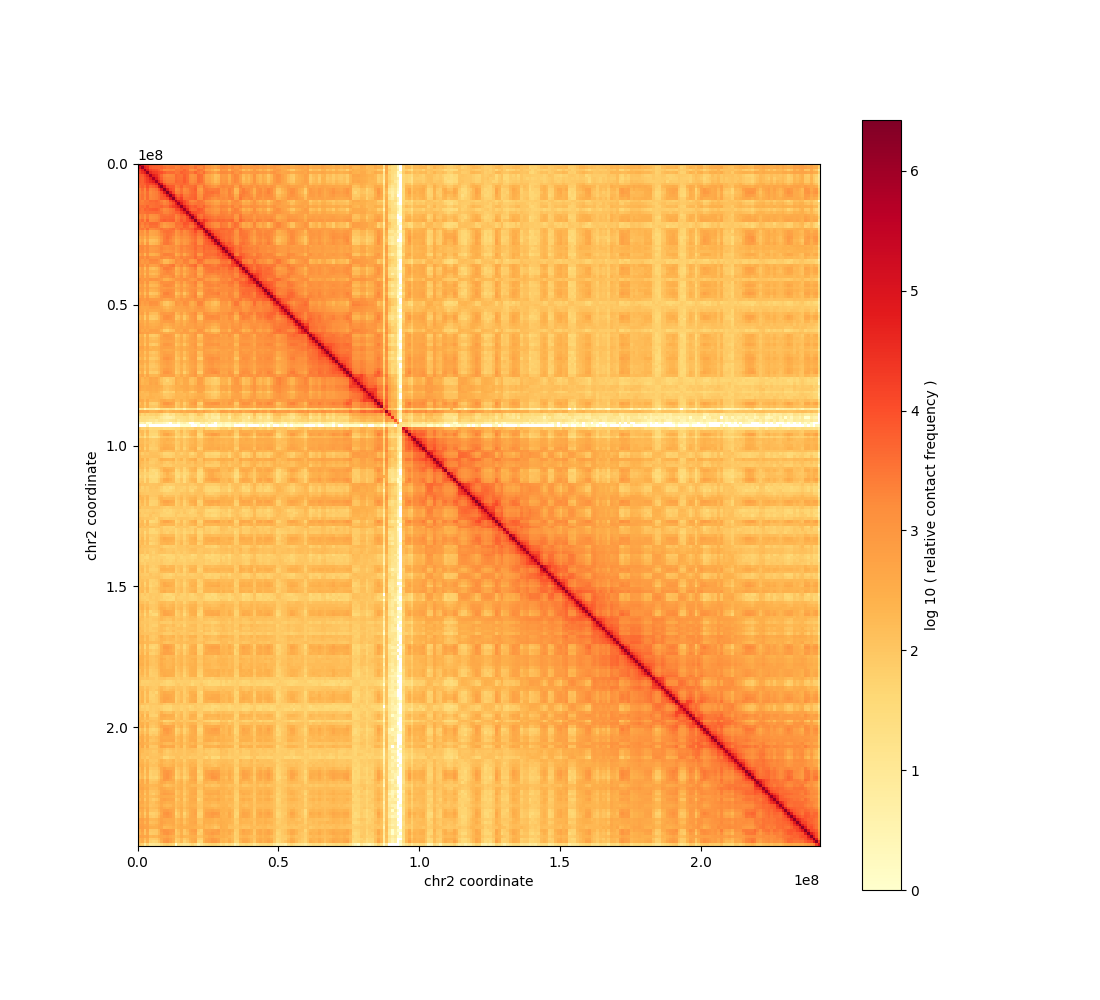
!cooler show $cool_file::resolutions/1000000 'chr2' -o 'outputs/chr2.png'
Traceback (most recent call last):
  File "/Users/geofffudenberg/anaconda3/envs/open2c/bin/cooler", line 8, in <module>
    sys.exit(cli())
  File "/Users/geofffudenberg/anaconda3/envs/open2c/lib/python3.9/site-packages/click/core.py", line 1130, in __call__
    return self.main(*args, **kwargs)
  File "/Users/geofffudenberg/anaconda3/envs/open2c/lib/python3.9/site-packages/click/core.py", line 1055, in main
    rv = self.invoke(ctx)
  File "/Users/geofffudenberg/anaconda3/envs/open2c/lib/python3.9/site-packages/click/core.py", line 1657, in invoke
    return _process_result(sub_ctx.command.invoke(sub_ctx))
  File "/Users/geofffudenberg/anaconda3/envs/open2c/lib/python3.9/site-packages/click/core.py", line 1404, in invoke
    return ctx.invoke(self.callback, **ctx.params)
  File "/Users/geofffudenberg/anaconda3/envs/open2c/lib/python3.9/site-packages/click/core.py", line 760, in invoke
    return __callback(*args, **kwargs)
  File "/Users/geofffudenberg/anaconda3/envs/open2c/lib/python3.9/site-packages/cooler/cli/show.py", line 230, in show
    plt.gcf().canvas.set_window_title("Contact matrix".format())
AttributeError: 'FigureCanvasAgg' object has no attribute 'set_window_title'
[6]:
Image('outputs/chr2.png', width=400, height=400)
[6]:
Expected
Tables of expected counts, either in cis or trans, are key inputs for many downstream analyses in cooltools. For more details, see the contacts_vs_dist notebook.
Typically, we specify a view to define regions under analysis. Here we quickly create a view that specifies chromosome arms using tables of chromosome sizes and centromere positions.
[7]:
# create a view of hg38 chromosome arms using chromosome sizes and definition of centromeres
hg38_chromsizes = bioframe.fetch_chromsizes('hg38')
hg38_cens = bioframe.fetch_centromeres('hg38')
view_hg38 = bioframe.make_chromarms(hg38_chromsizes,  hg38_cens)

# select only those chromosomes available in cooler
clr = cooler.Cooler(f'{cool_file}::/resolutions/1000000')
view_hg38 = view_hg38[view_hg38.chrom.isin(clr.chromnames)].reset_index(drop=True)
view_hg38.to_csv("data/view_hg38.tsv", index=False, header=False, sep='\t')
[8]:
! cooltools expected-cis $cool_file::resolutions/100000 --nproc 6 -o 'outputs/test.expected.cis.100000.tsv' --view "data/view_hg38.tsv"
Note expected for the first two distances are not defined with default settings, due to masking of near-diagonals in the cooler.
[9]:
display(
    pd.read_table("outputs/test.expected.cis.100000.tsv")[0:5]
)
| region1 | region2 | dist | n_valid | count.sum | balanced.sum | count.avg | balanced.avg | |
|---|---|---|---|---|---|---|---|---|
| 0 | chr2_p | chr2_p | 0 | 878 | NaN | NaN | NaN | NaN |
| 1 | chr2_p | chr2_p | 1 | 876 | NaN | NaN | NaN | NaN |
| 2 | chr2_p | chr2_p | 2 | 874 | 2738583.0 | 65.287351 | 3133.390160 | 0.074699 |
| 3 | chr2_p | chr2_p | 3 | 872 | 1739972.0 | 41.011675 | 1995.380734 | 0.047032 |
| 4 | chr2_p | chr2_p | 4 | 870 | 1184707.0 | 28.473626 | 1361.732184 | 0.032728 |
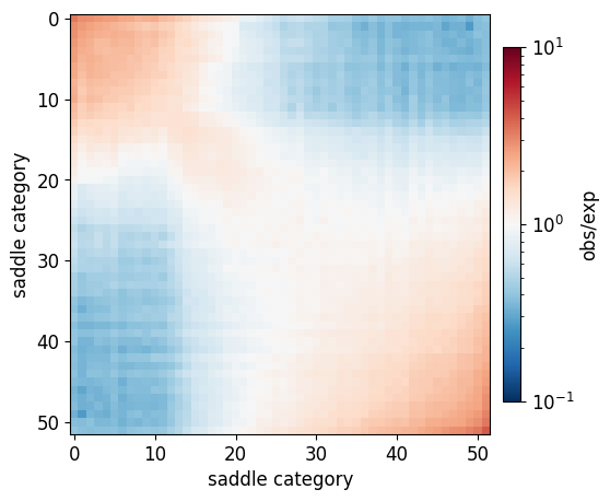
Compartments & saddles
Many contact maps display plaid patterns of interactions. For more detail see the compartments notebook.
Since the orientation of eigenvectors is determined up to a sign, we often use GC content to orient or “phase” eigenvectors. Before calculating comparments, this notebook generates a binned GC content profile for the relevant region.
[10]:
## fasta sequence is required for calculating binned profile of GC conent
if not os.path.isfile('./data/hg38.fa'):
    ## note downloading a ~1Gb file can take a minute
    subprocess.call('wget -P ./data --progress=bar:force:noscroll https://hgdownload.cse.ucsc.edu/goldenpath/hg38/bigZips/hg38.fa.gz', shell=True)
    subprocess.call('gunzip ./data/hg38.fa.gz', shell=True)
Bins can be fetched from the cooler, dropping any weights columns & keeping the header.
[11]:
!cooler dump --header -t bins $cool_file::resolutions/100000 | cut -f1-3 > outputs/bins.100000.tsv
[12]:
!cooltools genome gc outputs/bins.100000.tsv data/hg38.fa > outputs/gc.100000.tsv
[13]:
!cooltools eigs-cis -o outputs/test.eigs.100000 --view data/view_hg38.tsv --phasing-track outputs/gc.100000.tsv --n-eigs 1 $cool_file::resolutions/100000
/Users/geofffudenberg/anaconda3/envs/open2c/lib/python3.9/site-packages/cooltools/lib/checks.py:550: FutureWarning: In a future version of pandas, a length 1 tuple will be returned when iterating over a groupby with a grouper equal to a list of length 1. Don't supply a list with a single grouper to avoid this warning.
  for name, group in track.groupby([track.columns[0]]):
[14]:
display(
    pd.read_table('outputs/test.eigs.100000.cis.vecs.tsv')[0:5]
)
| chrom | start | end | weight | E1 | |
|---|---|---|---|---|---|
| 0 | chr2 | 0 | 100000 | 0.006754 | -1.564658 |
| 1 | chr2 | 100000 | 200000 | 0.006767 | -1.747567 |
| 2 | chr2 | 200000 | 300000 | 0.004638 | -0.370827 |
| 3 | chr2 | 300000 | 400000 | 0.006034 | -1.326894 |
| 4 | chr2 | 400000 | 500000 | 0.006153 | -1.434981 |
Pairwise class averaging is a typical way to reveal preferences in contact frequencies between regions.
[15]:
!cooltools saddle --qrange 0.02 0.98 --fig png -o outputs/test.saddle.cis.100000 --view data/view_hg38.tsv $cool_file::resolutions/100000 outputs/test.eigs.100000.cis.vecs.tsv outputs/test.expected.cis.100000.tsv
/Users/geofffudenberg/anaconda3/envs/open2c/lib/python3.9/site-packages/cooltools/lib/checks.py:550: FutureWarning: In a future version of pandas, a length 1 tuple will be returned when iterating over a groupby with a grouper equal to a list of length 1. Don't supply a list with a single grouper to avoid this warning.
  for name, group in track.groupby([track.columns[0]]):
[16]:
saddle = np.load('outputs/test.saddle.cis.100000.saddledump.npz', allow_pickle=True)
[17]:
plt.figure(figsize=(6,6))
norm = LogNorm(    vmin=10**(-1), vmax=10**1)
im = plt.imshow(
    saddle['saddledata'],
    cmap='RdBu_r',
    norm = norm
);
plt.xlabel("saddle category")
plt.ylabel("saddle category")
plt.colorbar(im, label='obs/exp', pad=0.025, shrink=0.7);
Insulation & boundaries
A common strategy to summarize the near-diagonal structure of a contact map is by computing insulation scores. See the insulation notebook for more details.
The command below uses the Li method to threshold the insulation score for boundary calling, so the resulting table has both log2 insulation scores and whether a given region is a boundary. The boundary_strength_{window} column has a value for all local minima of the insulation profile, and the is_boundary_{window} column indicates whether this strength passed the threshold. Note that {window} indicates the chosen size of the sliding diamond, and the command below uses windows of size 100kb and 200kb.
[18]:
! cooltools insulation --threshold Li -o 'outputs/test.insulation.10000.tsv' --view "data/view_hg38.tsv" $cool_file::resolutions/10000 100000 200000
[19]:
display(
    pd.read_table('outputs/test.insulation.10000.tsv')[0:5]
)
| chrom | start | end | region | is_bad_bin | log2_insulation_score_100000 | n_valid_pixels_100000 | log2_insulation_score_200000 | n_valid_pixels_200000 | boundary_strength_100000 | boundary_strength_200000 | is_boundary_100000 | is_boundary_200000 | |
|---|---|---|---|---|---|---|---|---|---|---|---|---|---|
| 0 | chr2 | 0 | 10000 | chr2_p | True | NaN | 0.0 | NaN | 0.0 | NaN | NaN | False | False |
| 1 | chr2 | 10000 | 20000 | chr2_p | False | 0.692051 | 8.0 | 1.123245 | 18.0 | NaN | NaN | False | False |
| 2 | chr2 | 20000 | 30000 | chr2_p | False | 0.760561 | 17.0 | 1.196643 | 37.0 | NaN | NaN | False | False |
| 3 | chr2 | 30000 | 40000 | chr2_p | False | 0.766698 | 27.0 | 1.211748 | 57.0 | NaN | NaN | False | False |
| 4 | chr2 | 40000 | 50000 | chr2_p | False | 0.674906 | 37.0 | 1.135037 | 77.0 | NaN | NaN | False | False |
Dots & focal enrichment
Punctate pairwise peaks of enriched contact frequency are a prevalent feature of mammalian interphase contact maps. See the dots notebook for more details.
Since dots are evident at higher resolutions, we first calculate the 10kb expected, and we used multiple cores to speed up the calculation.
[20]:
! cooltools expected-cis --nproc 6 -o 'outputs/test.expected.cis.10000.tsv' --view "data/view_hg38.tsv" $cool_file::resolutions/10000
[21]:
! cooltools dots --nproc 6 -o 'outputs/test.dots.10000.tsv' --view "data/view_hg38.tsv" $cool_file::resolutions/10000 outputs/test.expected.cis.10000.tsv
INFO:root:Using recommended donut-based kernels with w=5, p=2 for binsize=10000
INFO:root: matrix 9314X9314 to be split into 256 tiles of 600X600.
INFO:root: tiles are padded (width=5) to enable convolution near the edges
INFO:root: matrix 14907X14907 to be split into 625 tiles of 600X600.
INFO:root: tiles are padded (width=5) to enable convolution near the edges
INFO:root: matrix 2472X2472 to be split into 25 tiles of 600X600.
INFO:root: tiles are padded (width=5) to enable convolution near the edges
INFO:root: matrix 5855X5855 to be split into 100 tiles of 600X600.
INFO:root: tiles are padded (width=5) to enable convolution near the edges
INFO:root:convolving 108 tiles to build histograms for lambda-bins
INFO:root:creating a Pool of 6 workers to tackle 108 tiles
INFO:root:Done building histograms in 17.489 sec ...
INFO:root:Determined thresholds for every lambda-bin ...
INFO:root:convolving 108 tiles to extract enriched pixels
INFO:root:creating a Pool of 6 workers to tackle 108 tiles
INFO:root:Done extracting enriched pixels in 18.971 sec ...
INFO:root:Begin post-processing of 11284 filtered pixels
INFO:root:preparing to extract needed q-values ...
INFO:root:clustering enriched pixels in region: chr17_p
INFO:root:detected 198 clusters of 3.69+/-3.15 size
INFO:root:clustering enriched pixels in region: chr17_q
INFO:root:detected 584 clusters of 3.87+/-3.44 size
INFO:root:clustering enriched pixels in region: chr2_p
INFO:root:detected 841 clusters of 3.82+/-3.56 size
INFO:root:clustering enriched pixels in region: chr2_q
INFO:root:detected 1364 clusters of 3.72+/-3.24 size
INFO:root:Clustering is complete
INFO:root:filtered 2548 out of 2987 centroids to reduce the number of false-positives
[22]:
display(
    pd.read_table('outputs/test.dots.10000.tsv')[0:5]
)
| chrom1 | start1 | end1 | chrom2 | start2 | end2 | count | la_exp.donut.value | la_exp.vertical.value | la_exp.horizontal.value | ... | la_exp.vertical.qval | la_exp.horizontal.qval | la_exp.lowleft.qval | region | cstart1 | cstart2 | c_label | c_size | region1 | region2 | |
|---|---|---|---|---|---|---|---|---|---|---|---|---|---|---|---|---|---|---|---|---|---|
| 0 | chr17 | 12250000 | 12260000 | chr17 | 12740000 | 12750000 | 186 | 72.485199 | 79.603089 | 72.129599 | ... | 2.210430e-22 | 2.032096e-22 | 1.506741e-33 | chr17_p | 1.220571e+07 | 1.273857e+07 | 0 | 7 | chr17_p | chr17_p |
| 1 | chr17 | 10640000 | 10650000 | chr17 | 11980000 | 11990000 | 64 | 20.549081 | 23.891314 | 25.102296 | ... | 1.368050e-08 | 1.294897e-08 | 8.847705e-09 | chr17_p | 1.063000e+07 | 1.195500e+07 | 1 | 4 | chr17_p | chr17_p |
| 2 | chr17 | 9920000 | 9930000 | chr17 | 10610000 | 10620000 | 444 | 40.054241 | 75.104470 | 41.227788 | ... | 3.310219e-171 | 7.071107e-246 | 2.515747e-246 | chr17_p | 9.920000e+06 | 1.061200e+07 | 2 | 4 | chr17_p | chr17_p |
| 3 | chr17 | 10640000 | 10650000 | chr17 | 10840000 | 10850000 | 340 | 34.137182 | 46.658333 | 48.204555 | ... | 2.637572e-154 | 1.768044e-154 | 4.524004e-183 | chr17_p | 1.063667e+07 | 1.083889e+07 | 3 | 9 | chr17_p | chr17_p |
| 4 | chr17 | 12180000 | 12190000 | chr17 | 13000000 | 13010000 | 215 | 28.235042 | 36.990608 | 38.266379 | ... | 7.841810e-80 | 1.045765e-79 | 7.967002e-80 | chr17_p | 1.218571e+07 | 1.299143e+07 | 4 | 7 | chr17_p | chr17_p |
5 rows × 22 columns
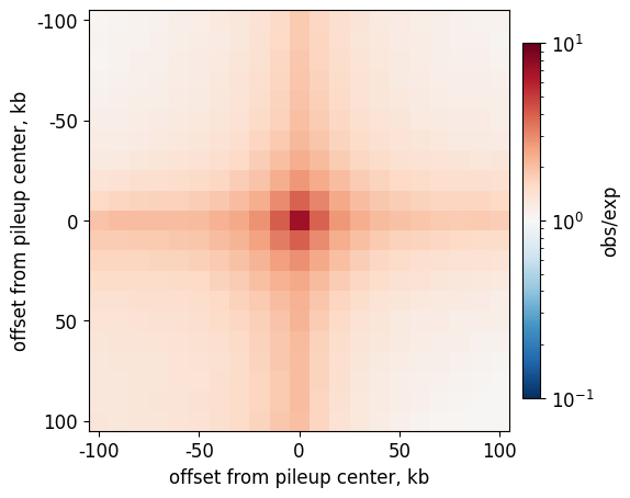
Pileups & average features
A common method for quantifying contact maps is by creating pileup plots, which are averages over a set of “snippets”, or 2D windows, from the genome-wide map. See the pileups notebook for more details.
Below shows pileup for dots that were computed above.
[23]:
!cooltools pileup --features-format BEDPE --nproc 6 -o 'outputs/test.pileup.10000.npz' --view "data/view_hg38.tsv" --expected outputs/test.expected.cis.10000.tsv $cool_file::resolutions/10000 outputs/test.dots.10000.tsv
[24]:
## output is saved as an npz with keys 'pileup' and 'stack'
resolution = 10000
pile = np.load( f'outputs/test.pileup.{resolution}.npz')
[25]:
plt.figure(figsize=(6,6))
norm = LogNorm(    vmin=10**(-1), vmax=10**1)

im = plt.imshow(
    pile['pileup'],
    cmap='RdBu_r',
    norm = norm
);

plt.xticks(np.arange(0,25,5).astype(int),
           (np.arange(0,25,5).astype(int)-10)*resolution//1000,
)
plt.yticks(np.arange(0,25,5).astype(int),
           (np.arange(0,25,5).astype(int)-10)*resolution//1000,
)
plt.xlabel("offset from pileup center, kb")
plt.ylabel("offset from pileup center, kb")

plt.colorbar(im, label='obs/exp', pad=0.025, shrink=0.7);
This page was generated with nbsphinx from /home/docs/checkouts/readthedocs.org/user_builds/cooltools/checkouts/latest/docs/notebooks/command_line_interface.ipynb