Insulation & boundaries

Welcome to the contact insulation notebook!

Insulation is a simple concept, yet a powerful way to look at C data. Insulation is one aspect of locus-specific contact frequency at small genomic distances, and reflects the segmentation of the genome into domains.

Insulation can be computed with multiple methods. One of the most common methods involves using a diamond-window score to generate an insulation profile. To compute this profile, slide a diamond-shaped window along the genome, with one of the corners on the main diagonal of the matrix, and sum up the contacts within the window for each position.

Insulation profiles reveal that certain locations have lower scores, reflecting lowered contact frequencies between upstream and downstream loci. These positions are often referred to as boundaries, and are also obtained with multiple methods. Here we illustrate one thresholding method for determining boundaries from an insulation profile.

In this notebook we:

• Calculate the insulation score genome-wide and display it alongside an interaction matrix

• Call insulating boundaries

• Filter insulating boundaries based on their strength

• Calculate enrichment of CTCF/genes at boundaries

• Repeat boundary filtering based on enrichmnent of CTCF, a known insulator protein in mammalian genomes

# import standard python libraries
import numpy as np
import matplotlib.pyplot as plt
import pandas as pd

# Import python package for working with cooler files and tools for analysis
import cooler
import cooltools.lib.plotting
from cooltools import insulation

from packaging import version
if version.parse(cooltools.__version__) < version.parse('0.5.4'):
    raise AssertionError("tutorials rely on cooltools version 0.5.4 or higher,"+
                         "please check your cooltools version and update to the latest")

# download test data
# this file is 145 Mb, and may take a few seconds to download
import cooltools
data_dir = './data/'
cool_file = cooltools.download_data("HFF_MicroC", cache=True, data_dir=data_dir)
print(cool_file)

./data/test.mcool

Calculating genome-wide contact insulation

Here we load the Hi-C data at 10 kbp resolution and calculate insulation score with 4 different window sizes

resolution = 10000
clr = cooler.Cooler(f'{data_dir}test.mcool::resolutions/{resolution}')
windows = [3*resolution, 5*resolution, 10*resolution, 25*resolution]
insulation_table = insulation(clr, windows, verbose=True)

INFO:root:fallback to serial implementation.
INFO:root:Processing region chr2
INFO:root:Processing region chr17

This function returns a dataframe where rows correspond to genomic bins of the cooler.

The columns of this insulation dataframe report the insulation score, the number of valid (non-nan) pixels, whether the given bin is valid, the boundary prominence (strength) and whether locus is called as a boundary after thresholding, for each of the window sizes provided to the function.

Below we print the information returned for any window size, as well as the specific information for the largest window used:

first_window_summary =insulation_table.columns[[ str(windows[-1]) in i for i in insulation_table.columns]]

insulation_table[['chrom','start','end','region','is_bad_bin']+list(first_window_summary)].iloc[1000:1005]

	chrom	start	end	region	is_bad_bin	log2_insulation_score_250000	n_valid_pixels_250000	boundary_strength_250000	is_boundary_250000
1000	chr2	10000000	10010000	chr2	False	0.309791	622.0	NaN	False
1001	chr2	10010000	10020000	chr2	False	0.226045	622.0	NaN	False
1002	chr2	10020000	10030000	chr2	False	0.090809	622.0	NaN	False
1003	chr2	10030000	10040000	chr2	False	-0.101091	622.0	NaN	False
1004	chr2	10040000	10050000	chr2	False	-0.342858	622.0	NaN	False

# Functions to help with plotting
def pcolormesh_45deg(ax, matrix_c, start=0, resolution=1, *args, **kwargs):
    start_pos_vector = [start+resolution*i for i in range(len(matrix_c)+1)]
    import itertools
    n = matrix_c.shape[0]
    t = np.array([[1, 0.5], [-1, 0.5]])
    matrix_a = np.dot(np.array([(i[1], i[0])
                                for i in itertools.product(start_pos_vector[::-1],
                                                           start_pos_vector)]), t)
    x = matrix_a[:, 1].reshape(n + 1, n + 1)
    y = matrix_a[:, 0].reshape(n + 1, n + 1)
    im = ax.pcolormesh(x, y, np.flipud(matrix_c), *args, **kwargs)
    im.set_rasterized(True)
    return im

from matplotlib.ticker import EngFormatter
bp_formatter = EngFormatter('b')
def format_ticks(ax, x=True, y=True, rotate=True):
    if y:
        ax.yaxis.set_major_formatter(bp_formatter)
    if x:
        ax.xaxis.set_major_formatter(bp_formatter)
        ax.xaxis.tick_bottom()
    if rotate:
        ax.tick_params(axis='x',rotation=45)

Let’s see what the insulation track at the highest resolution looks like, next to a rotated Hi-C matrix.

from matplotlib.colors import LogNorm
from mpl_toolkits.axes_grid1 import make_axes_locatable
import bioframe
plt.rcParams['font.size'] = 12

start = 10_500_000
end = start+ 90*windows[0]
region = ('chr2', start, end)
norm = LogNorm(vmax=0.1, vmin=0.001)
data = clr.matrix(balance=True).fetch(region)
f, ax = plt.subplots(figsize=(18, 6))
im = pcolormesh_45deg(ax, data, start=region[1], resolution=resolution, norm=norm, cmap='fall')
ax.set_aspect(0.5)
ax.set_ylim(0, 10*windows[0])
format_ticks(ax, rotate=False)
ax.xaxis.set_visible(False)

divider = make_axes_locatable(ax)
cax = divider.append_axes("right", size="1%", pad=0.1, aspect=6)
plt.colorbar(im, cax=cax)

insul_region = bioframe.select(insulation_table, region)

ins_ax = divider.append_axes("bottom", size="50%", pad=0., sharex=ax)
ins_ax.set_prop_cycle(plt.cycler("color", plt.cm.plasma(np.linspace(0,1,5))))
ins_ax.plot(insul_region[['start', 'end']].mean(axis=1),
            insul_region['log2_insulation_score_'+str(windows[0])],
            label=f'Window {windows[0]} bp')

ins_ax.legend(bbox_to_anchor=(0., -1), loc='lower left', ncol=4);

format_ticks(ins_ax, y=False, rotate=False)
ax.set_xlim(region[1], region[2])

(10500000.0, 13200000.0)

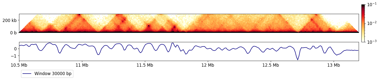
And now let’s add the other window sizes.

for res in windows[1:]:
    ins_ax.plot(insul_region[['start', 'end']].mean(axis=1), insul_region[f'log2_insulation_score_{res}'], label=f'Window {res} bp')
ins_ax.legend(bbox_to_anchor=(0., -1), loc='lower left', ncol=4);
f

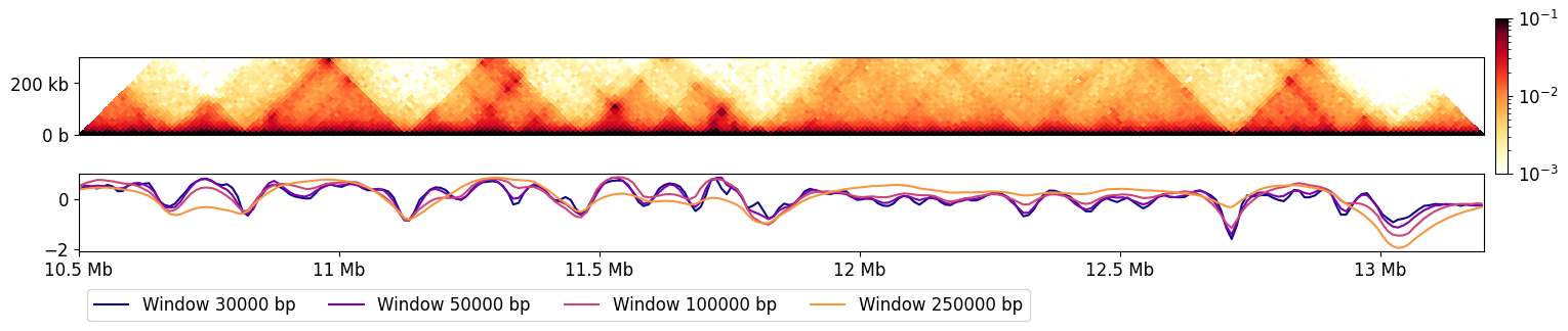
This really highlights how much the result is dependent on window size: smaller windows are sensitive to local structure, whereas large windows capture regions that insulate at larger scales.

Boundary calling

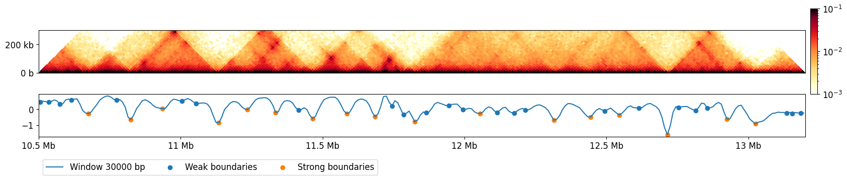
The insulation table also has annotations for valleys of the insulation score, which correspond to highly insulating regions, such as TAD boundaries. All potential boundaries have an assigned boundary_strength_ column. Additionally, this strength is thresholded to find regions that insulate particularly strongly, and this is recorded in the is_boundary_ columns.

Let’s repeat the previous plot and show where we found the boundaries:

f, ax = plt.subplots(figsize=(20, 10))
im = pcolormesh_45deg(ax, data, start=region[1], resolution=resolution, norm=norm, cmap='fall')
ax.set_aspect(0.5)
ax.set_ylim(0, 10*windows[0])
format_ticks(ax, rotate=False)
ax.xaxis.set_visible(False)

divider = make_axes_locatable(ax)
cax = divider.append_axes("right", size="1%", pad=0.1, aspect=6)
plt.colorbar(im, cax=cax)

insul_region = bioframe.select(insulation_table, region)

ins_ax = divider.append_axes("bottom", size="50%", pad=0., sharex=ax)

ins_ax.plot(insul_region[['start', 'end']].mean(axis=1),
            insul_region[f'log2_insulation_score_{windows[0]}'], label=f'Window {windows[0]} bp')

boundaries = insul_region[~np.isnan(insul_region[f'boundary_strength_{windows[0]}'])]
weak_boundaries = boundaries[~boundaries[f'is_boundary_{windows[0]}']]
strong_boundaries = boundaries[boundaries[f'is_boundary_{windows[0]}']]
ins_ax.scatter(weak_boundaries[['start', 'end']].mean(axis=1),
            weak_boundaries[f'log2_insulation_score_{windows[0]}'], label='Weak boundaries')
ins_ax.scatter(strong_boundaries[['start', 'end']].mean(axis=1),
            strong_boundaries[f'log2_insulation_score_{windows[0]}'], label='Strong boundaries')

ins_ax.legend(bbox_to_anchor=(0., -1), loc='lower left', ncol=4);

format_ticks(ins_ax, y=False, rotate=False)
ax.set_xlim(region[1], region[2])

(10500000.0, 13200000.0)

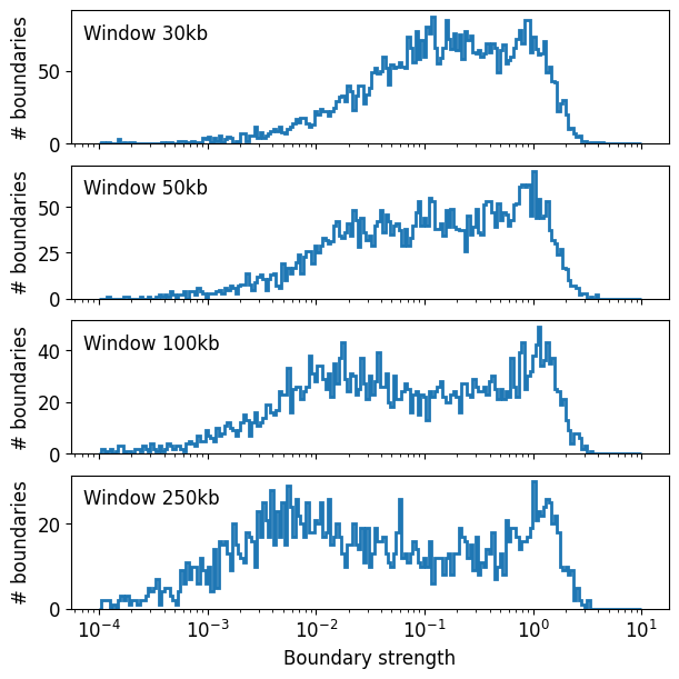
Calculating boundary strength

Let’s inspect the histogram of boundary strengths to show how we selected the strong boundaries.

First, boundary strength is calculated using the peak prominence, on the dips (or minima) of the insulation profile.

histkwargs = dict(
    bins=10**np.linspace(-4,1,200),
    histtype='step',
    lw=2,
)

f, axs = plt.subplots(len(windows),1, sharex=True, figsize=(6,6), constrained_layout=True)
for i, (w, ax) in enumerate(zip(windows, axs)):
    ax.hist(
        insulation_table[f'boundary_strength_{w}'],
        **histkwargs
    )
    ax.text(0.02, 0.9,
             f'Window {w//1000}kb',
             ha='left',
             va='top',
             transform=ax.transAxes)

    ax.set(
        xscale='log',
        ylabel='# boundaries'
    )

axs[-1].set(xlabel='Boundary strength');

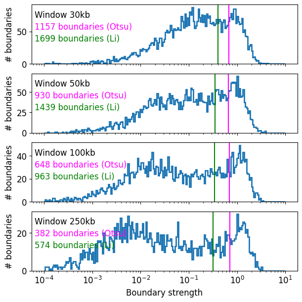
As a quick way to automatically threshold the histogram, we borrow the tresholding methods from the image analysis field. These include Li (default threshold="Li") or Otsu, as implemented in scikit-image. Otsu is more conservative, whereas Li is more permissive.

In practice these thresholds work well for a simple parameter-free method for mammalian interphase data, though should be double-checked for any individual dataset.

from skimage.filters import threshold_li, threshold_otsu

f, axs = plt.subplots(len(windows), 1, sharex=True, figsize=(6,6), constrained_layout=True)
thresholds_li = {}
thresholds_otsu = {}
for i, (w, ax) in enumerate(zip(windows, axs)):
    ax.hist(
        insulation_table[f'boundary_strength_{w}'],
        **histkwargs
    )
    thresholds_li[w] = threshold_li(insulation_table[f'boundary_strength_{w}'].dropna().values)
    thresholds_otsu[w] = threshold_otsu(insulation_table[f'boundary_strength_{w}'].dropna().values)
    n_boundaries_li = (insulation_table[f'boundary_strength_{w}'].dropna()>=thresholds_li[w]).sum()
    n_boundaries_otsu = (insulation_table[f'boundary_strength_{w}'].dropna()>=thresholds_otsu[w]).sum()
    ax.axvline(thresholds_li[w], c='green')
    ax.axvline(thresholds_otsu[w], c='magenta')
    ax.text(0.01, 0.9,
             f'Window {w//1000}kb',
             ha='left',
             va='top',
             transform=ax.transAxes)
    ax.text(0.01, 0.7,
            f'{n_boundaries_otsu} boundaries (Otsu)',
            c='magenta',
            ha='left',
            va='top',
            transform=ax.transAxes)
    ax.text(0.01, 0.5,
            f'{n_boundaries_li} boundaries (Li)',
            c='green',
            ha='left',
            va='top',
            transform=ax.transAxes)

    ax.set(
        xscale='log',
        ylabel='# boundaries'
    )

axs[-1].set(xlabel='Boundary strength')

[Text(0.5, 0, 'Boundary strength')]

CTCF enrichment at boundaries

TAD boundaries are frequently associated with CTCF binding.

To quantify this, we can aggregate the ChIP-Seq singal around the boundaries, and compare enrichment of CTCF with boundary strength using pybbi (https://github.com/nvictus/pybbi). We provide a test bigWig file with CTCF enrichment over input for the same cell type as the Micro-C data.

We use the bbi.stackup() method with no binning to extract an array of average values for all boundary regions with 1 kbp flanks.

# Download test data. The file size is 592 Mb, so the download might take a while:
ctcf_fc_file = cooltools.download_data("HFF_CTCF_fc", cache=True, data_dir=data_dir)

import bbi

is_boundary = np.any([
        ~insulation_table[f'boundary_strength_{w}'].isnull()
        for w in windows],
    axis=0)
boundaries = insulation_table[is_boundary]
boundaries.head()

	chrom	start	end	region	is_bad_bin	log2_insulation_score_30000	n_valid_pixels_30000	log2_insulation_score_50000	n_valid_pixels_50000	log2_insulation_score_100000	...	log2_insulation_score_250000	n_valid_pixels_250000	boundary_strength_30000	boundary_strength_50000	boundary_strength_250000	boundary_strength_100000	is_boundary_30000	is_boundary_50000	is_boundary_100000	is_boundary_250000
5	chr2	50000	60000	chr2	False	0.089080	6.0	0.059578	22.0	0.586104	...	1.211581	122.0	NaN	0.156397	NaN	NaN	False	False	False	False
6	chr2	60000	70000	chr2	False	0.036906	6.0	0.134037	22.0	0.547732	...	1.161302	147.0	0.150452	NaN	NaN	NaN	False	False	False	False
7	chr2	70000	80000	chr2	False	0.062353	6.0	0.122444	22.0	0.479052	...	1.092480	172.0	NaN	0.011593	NaN	NaN	False	False	False	False
9	chr2	90000	100000	chr2	False	0.049426	6.0	0.198381	22.0	0.377645	...	0.972715	222.0	0.029686	NaN	NaN	NaN	False	False	False	False
11	chr2	110000	120000	chr2	False	0.095762	6.0	0.190455	22.0	0.320182	...	0.867080	272.0	NaN	0.024922	NaN	NaN	False	False	False	False

5 rows × 21 columns

# Calculate the average ChIP singal/input in the 3kb region around the boundary.
flank = 1000 # Length of flank to one side from the boundary, in basepairs
ctcf_chip_signal = bbi.stackup(
    data_dir+'/test_CTCF.bigWig',
    boundaries.chrom,
    boundaries.start-flank,
    boundaries.end+flank,
    bins=1).flatten()

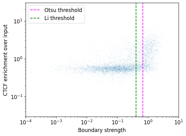
Real boundaries are often enriched in CTCF binding, and this can be used as a guide for thresholding the boundary strength. However note a small population of strong boundaries without CTCF binding.

w=windows[0]
f, ax = plt.subplots()
ax.loglog(
    boundaries[f'boundary_strength_{w}'],
    ctcf_chip_signal,
    'o',
    markersize=1,
    alpha=0.05
);
ax.set(
    xlim=(1e-4,1e1),
    ylim=(3e-2,3e1),
    xlabel='Boundary strength',
    ylabel='CTCF enrichment over input')

ax.axvline(thresholds_otsu[w], ls='--', color='magenta', label='Otsu threshold')
ax.axvline(thresholds_li[w], ls='--', color='green', label='Li threshold')
ax.legend()

<matplotlib.legend.Legend at 0x1afd95dc0>

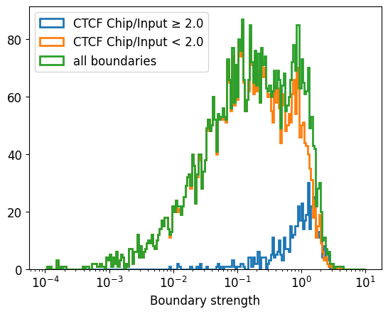
If we were interested specifically in boundaries with CTCF, we could threshold based on enrichment of CTCF ChIP-seq:

histkwargs = dict(
    bins=10**np.linspace(-4,1,200),
    histtype='step',
    lw=2,
)
f, ax = plt.subplots()
ax.set(xscale='log', xlabel='Boundary strength')
ax.hist(
    boundaries[f'boundary_strength_{windows[0]}'][ctcf_chip_signal>=2],
    label='CTCF Chip/Input ≥ 2.0',
    **histkwargs
);
ax.hist(
    boundaries[f'boundary_strength_{windows[0]}'][ctcf_chip_signal<2],
    label='CTCF Chip/Input < 2.0',
    **histkwargs
);
ax.hist(
    boundaries[f'boundary_strength_{windows[0]}'],
    label='all boundaries',
    **histkwargs
);
ax.legend(loc='upper left')

<matplotlib.legend.Legend at 0x1af14eac0>

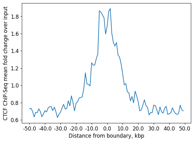
1D pileup: CTCF enrichment at boundaries

Additionally, we can create 1D pileup plot of average CTCF enrichment.

First, create a collection of genomic regions of equal size, each centered at the position of the boundary.

Then, create a stackup of binned ChIP-Seq signal for these regions. It is based on the same test bigWig file with the CTCF ChIP-Seq log fold change over input.

Finally, create 1D pileup by averaging each stacked window.

# Select the strict thresholded boundaries for one window size
top_boundaries = insulation_table[insulation_table[f'boundary_strength_{windows[1]}']>=thresholds_otsu[windows[1]]]

# Create of the stackup, the flanks are +- 50 Kb, number of bins is 100 :
flank = 50000 # Length of flank to one side from the boundary, in basepairs
nbins = 100   # Number of bins to split the region
stackup = bbi.stackup(data_dir+'/test_CTCF.bigWig',
                      top_boundaries.chrom,
                      top_boundaries.start+resolution//2-flank,
                      top_boundaries.start+resolution//2+flank,
                      bins=nbins)

f, ax = plt.subplots(figsize=[7,5])
ax.plot(np.nanmean(stackup, axis=0) )
ax.set(xticks=np.arange(0, nbins+1, 10),
       xticklabels=(np.arange(0, nbins+1, 10)-nbins//2)*flank*2/nbins/1000,
       xlabel='Distance from boundary, kbp',
       ylabel='CTCF ChIP-Seq mean fold change over input');

Using adjacent boundaries to create a table of TADs

Calling TADs from Hi-C data poses a challenge, in part because domain structures vary greatly in their size, intensity, and can be nested. The number of called TADs varies substantially from tool to tool, and can depend on tool-specific parameters (Forcato, 2017). Below, we show an example of how adjacent boundaries calculated with cooltools can specify a set of intervals that could be analyzed as TADs, using bioframe.merge().

def extract_TADs(insulation_table, is_boundary_col, max_TAD_length = 3_000_000):
    tads = bioframe.merge(insulation_table[insulation_table[is_boundary_col] == False])
    return tads[ (tads["end"] - tads["start"]) <= MAX_TAD_LENGTH].reset_index(drop=True)[['chrom','start','end']]

TADs_table = extract_TADs(insulation_table, f'is_boundary_{windows[0]}')
TADs_table.head()

TADs_table

	chrom	start	end
0	chr2	0	200000
1	chr2	210000	290000
2	chr2	300000	670000
3	chr2	680000	740000
4	chr2	750000	950000
...	...	...	...
1693	chr17	82460000	82640000
1694	chr17	82650000	82760000
1695	chr17	82770000	82960000
1696	chr17	82970000	83080000
1697	chr17	83090000	83257441

1698 rows × 3 columns

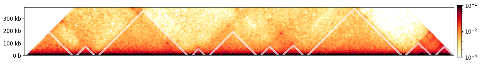
# Visualizing the first 10 inter-boundary intervals (grey overay) v.s. Hi-C data

region = ('chr2', TADs_table.iloc[0].start, TADs_table.iloc[9].end)
norm = LogNorm(vmax=0.1, vmin=0.001)
data = clr.matrix(balance=True).fetch(region)

f, ax = plt.subplots(figsize=(18, 6))
im = pcolormesh_45deg(ax, data, start=region[1], resolution=resolution, norm=norm, cmap='fall')
ax.set_aspect(0.5)
ax.set_ylim(0, 13*windows[0])
format_ticks(ax, rotate=False)
ax.xaxis.set_visible(False)

divider = make_axes_locatable(ax)
cax = divider.append_axes("right", size="1%", pad=0.1, aspect=6)
plt.colorbar(im, cax=cax)

idx = 10
max_pos = TADs_table[:idx]['end'].max()/resolution
contact_matrix = np.zeros((int(max_pos), int(max_pos)))
contact_matrix[:] = np.nan
for _, row in TADs_table[:idx].iterrows():
    contact_matrix[int(row['start']/resolution):int(row['end']/resolution), int(row['start']/resolution):int(row['end']/resolution)] = 1
    contact_matrix[int(row['start']/resolution + 1):int(row['end']/resolution - 1), int(row['start']/resolution + 1):int(row['end']/resolution - 1)] = np.nan

im = pcolormesh_45deg(ax, contact_matrix, start=0, resolution=resolution, cmap='gray', vmax=1, vmin=-1, alpha=0.6)

plt.show()

---

This page was generated with nbsphinx from /home/docs/checkouts/readthedocs.org/user_builds/cooltools/checkouts/latest/docs/notebooks/insulation_and_boundaries.ipynb